How Do You Know if a Function Is Differentiable on an Interval

Differentiability

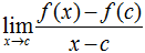
So far we take looked at derivatives outside of the notion of differentiability. The problem with this approach, though, is that some functions have i or many points or intervals where their derivatives are undefined. A function f is differentiable at a indicate c if

exists.

Similarly, f is differentiable on an open interval (a, b) if

exists for every c in (a, b).

Basically, f is differentiable at c if f'(c) is divers, by the above definition. Another point of note is that if f is differentiable at c, then f is continuous at c.

Let's go through a few examples and hash out their differentiability. First, consider the following function.

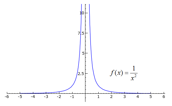
plot(i/x^2, x, -v, 5).show(ymin=0, ymax=10)        

Toggle Line Numbers

To observe the limit of the function's gradient when the alter in x is 0, we can either use the true definition of the derivative and practice

def f(ten):     render one/ten^2  var('h') ((f(x+h)-f(10))/h).rational_simplify().subs(h=0)        

Toggle Line Numbers

or we can simply utilise the rules of differentiation by calling 'derivative(one/x^2, x)'. In any case, we detect that

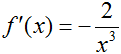
Since f'(x) is undefined when ten = 0 (-2/0² = ?), nosotros say that f is not differentiable at x = 0. Since f'(x) is defined for every other 10, nosotros can say that f' is continuous on (-∞, 0) U (0, ∞), where "U" denotes the union of 2 intervals.

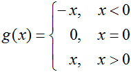
How about a function that is everywhere continuous but is not everywhere differentiable? This occurs quite often with piecewise functions, since even though two intervals might be connected, the slope can change radically at their junction. Take a look at the part g(x) = |ten|.

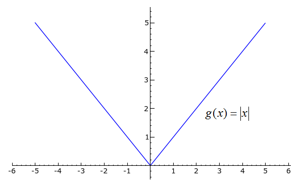
plot(abs(10), ten, -5, 5)        

Toggle Caption Toggle Line Numbers

1) Plot the absolute value of x from -5 to five.

Using our knowledge of what "absolute value" means, we can rewrite g(x) in the expanded grade

This should exist easy to differentiate now; we get

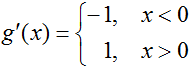
What well-nigh at x = 0? The "logical" response would be to encounter that g(0) = 0 and say that g'(0) must therefore equal 0. Careful, though...looking back at the limit definition of the derivative, the derivative of f at a point c is the limit of the slope of f as the alter in its independent variable approaches 0. Really, the only relevant piece of information is the behavior of function's slope close to c. Referring back to the example, since the limit of k'(x) as 10 approaches 0 from the left ≠ the limit of g'(x) as ten approaches 0 from the right, g'(0) does not be. We can use the limit definition of the derivative to testify this:

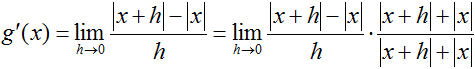
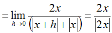
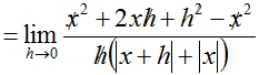
,  and then,  which is undefined.

In this form, it makes far more than sense why g'(0) is undefined. By simply looking at the graph of g, too, one tin can see that the sudden "twist" at ten = 0 is responsible for our disability to evaluate m' there. We can now justly pronounce that grand is differentiable on (-∞, 0) U (0, ∞), so 1000' is continuous on that same interval.

The third role of discussion has a couple of quirks--take a wait.

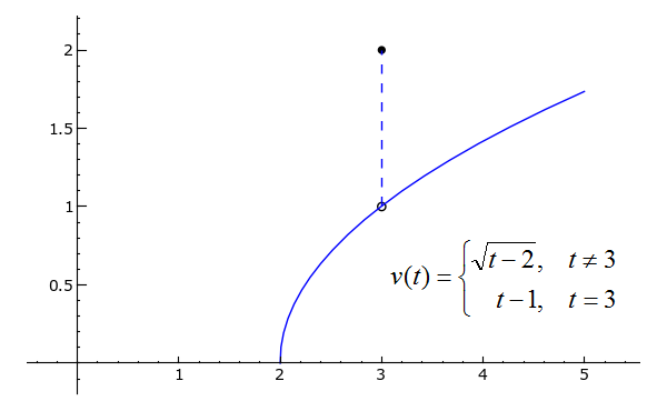
p = plot(sqrt(x-ii), x, ii, 5) pt1 = bespeak((3, 1), rgbcolor="white", pointsize=30, faceted=True) pt2 = point((3, two), rgbcolor="black", pointsize=30) l = line([(3, 1), (3, 2)], linestyle="--") (p+pt1+pt2+l).show(xmin=0)        

Toggle Line Numbers

Not but is v(t) defined solely on [2, ∞), it has a leap discontinuity at t = three. The jump aperture causes v'(t) to be undefined at t = three; do you see why? Using a slightly modified limit definition of the derivative, recall of what

would be for c = 3 and some x very close to three. The resulting gradient would be astronomically large either negatively or positively, correct? In fact, the dashed line connecting 5(t) for t ≠ 3 and v(3) is what the tangent line will look like at that point. Since a part's derivative cannot be infinitely large and nonetheless exist considered to "exist" at that bespeak, v is not differentiable at t=3.

The Mean Value Theorem

The Mean Value Theorem is very important for the word of derivatives; fifty-fifty though it might seem somewhat obvious, it is actually very important to many other concepts in calculus. We'll beginning with an example.

Consider the vast, seemingly countless country of Montana. Now, pretend that y'all are driving across Montana so that y'all can go to Washington, and you desire to do so every bit quickly every bit possible. The problem, notwithstanding, is that the signs posted every few miles explicitly state that the speed limit is 70 miles per hour. "Oh well," you tell yourself. "When I'm on the open road, I will get as fast equally I want. When I approach a town, though, I will slow down and then that the police are none the wiser."

Since you had been staying with some relatives in the town of Springdale, you showtime head eastward at the brisk pace of ninety miles per hour until, feeling your tum rumble (you actually aren't cutting out for these long drives), you stop in Livingston for some lunch. When y'all make it, however, a policeman signals you to pull over! "What did I do wrong?" yous sweetly enquire the officeholder. Giving you a difficult look, the policeman responds, "Though I didn't actually encounter yous speeding at any point on your mode hither, I know that y'all must have, since one of my buddies back in Livingston tells me that you left there only ten minutes ago, and our 2 towns are about xv miles apart. I won't cite yous for information technology this fourth dimension, but you'd improve bulldoze slower in the future."

The question is: How did the policeman know you had been speeding? Well, since it took yous ten minutes to travel 15 miles, your average speed was 90 miles per hour. And so either y'all traveled at exactly xc miles per hour the entire time, or you traveled at more than 90 part of the way and less than ninety function of the manner. In either example, you were going faster than the speed limit at some signal in time.

The Hateful Value Theorem has a very similar message: if a role f is continuous on the closed interval [a, b] and is differentiable on the open interval (a, b), then there is some c in (a, b) such that

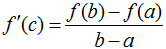
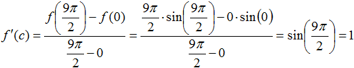
Basically, the average slope of f betwixt a and b will equal the actual slope of f at some point betwixt a and b. To illustrate the Mean Value Theorem, consider the office f(10) = x*sin(x) for x in [0, 9π/ii]. Presume that f is differentiable on (0, 9π/two) (it is) and continuous on [0, 9π/2] (it is). By the Mean Value Theorem, there is at least i c in (0, 9π/2) such that

.

And such a c does exist, in fact. Y'all can use SageMath'south solve part to verify this:

solve(derivative(x*sin(x), x) == 0, x)        

Toggle Line Numbers

From the code'south output, yous can see that this is true whenever -sin(x)/cos(10) is 0. Thus c = 0, π, 2π, 3π, and 4π, so the Mean Value Theorem is satisfied for f on the interval [0, 9π/ii].

Rolle's Theorem

Rolle's Theorem states that if a function thousand is differentiable on (a, b), continuous [a, b], and grand(a) = chiliad(b), then in that location is at least one number c in (a, b) such that chiliad'(c) = 0. To meet this, consider the everywhere differentiable and everywhere continuous function g(x) = (x-iii)*(x+2)*(10^2+4). To prove that thou' has at to the lowest degree ane zero for x in (-∞, ∞), notice that g(3) = thou(-2) = 0. By Rolle's Theorem, there must be at least one c in (-2, three) such that m'(c) = 0.

Practice Problems

Make up one's mind the interval(s) on which the following functions are continuous and the interval(s) on which they are differentiable.
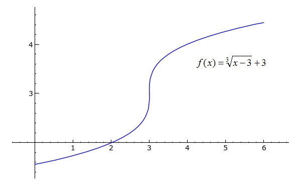
1)
Toggle answer

plot((x-three)^(1/iii)+3, ten, iii, 6) + plot(-(-x+3)^(1/3)+three, x, 0, iii)          

Toggle Explanation Toggle Line Numbers

1) Taking the cube root (or whatever odd root) of a negative number does non work well in Python, so one has to use multiple plot commands for functions such as x^(ane/three) to recoup for the intervals on which x is negative.

2)
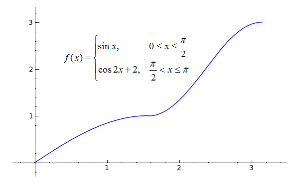
Hint: and so both pieces of f match at π/2? Exercise the derivatives of the two pieces lucifer there?
Toggle respond

plot(sin(x), x, 0, pi/2)+plot(cos(2*x)+2, x, pi/2, pi)          

Toggle Line Numbers
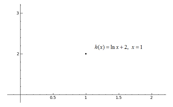
3)
Toggle answer

betoken((1, ln(1)+2), rgbcolor='black').testify()          

Toggle Line Numbers

---

Utilise the Mean Value Theorem to reply the following questions.

four) Marvin claims that he is a speed-walker and that he always walks at half dozen miles per hour. He tells yous that it took him simply 12 minutes to walk one mile this morning. Testify that Marvin was not actually speed-walking at some point during his walk.
Toggle answer

5) Jessica plays for a recreational basketball team, and has noticed an interesting trend: the number of points she scores each game has increased linearly for the first 5 games of the flavour. If she scored 10 points in the showtime game, must there be some game of the last five in which she scored 14 points?
Toggle answer

half dozen) Suppose that f'(ten) < 1 for 10 in (0, 4). If f(0) = 1, tin f(4) = 5?
Toggle reply

How Do You Know if a Function Is Differentiable on an Interval

Source: https://www.sagemath.org/calctut/differentiability.html

Share this post